Approaching geovisualization and remote sensing with GeoViews
Link: http://bit.ly/geopython-basel
09/05/2018 @ GeoPython
Giacomo Debidda
What is GeoViews?
A Python library that makes it easy to explore and visualize geographical, meteorological, oceanographic datasets.
- GIS extension for Holoviews
- Declarative API: annotate your data and let it visualize itself
- Uses Cartopy for geographic projections
- Uses Shapely for geometries
- Allows to create plots from multidimesional dataset (gridded dataset)
- Makes it easy to overlay layers in a visualization
- Leverages many Python libraries: Pandas, GeoPandas, Xarray, Datashader, Matplotlib/Bokeh
GeoViews objects
GeoViews objects are just like HoloViews objects...
...with an associated geographic projection based on a Coordinate Reference System defined in cartopy.crs.
GeoViews provides the Feature (cartopy features) and Shape (shapely geometries) types.
Imports
We need shapely for geometries, cartopy and pyproj for projections, geopandas for spatial joins.
import os
import pyproj
import numpy as np
import pandas as pd
import geopandas as gpd
import xarray as xr
import holoviews as hv
import geoviews as gv
import geoviews.feature as gf
import shapely as shp
import cartopy.io.shapereader as shpreader
import cartopy.crs as ccrs  # Cartopy coordinate reference system
import cartopy.feature as cf
import matplotlib.pyplot as plt
from bokeh.models import WMTSTileSource
from bokeh.tile_providers import STAMEN_TERRAIN, STAMEN_TONER
# import bokeh.sampledata
# bokeh.sampledata.download()  # this will download to /home/jack/.bokeh/data/
from bokeh.sampledata.airport_routes import airports, routes
data_dir = os.path.join(os.getcwd(), 'data')
print(data_dir)
Choose a plotting backend
GeoViews (and HoloViews) can use either a Matplotlib backend or a Bokeh backend.
- Matplotlib
- + supports more projections
- - less interactivity
- - at the moment, it seems not possible to use Web Map Tile Services (WMTS)
- Bokeh
- + better interactivity
- + can use Web Map Tile Services
- - supports only the Mercator projection
Note: visual attributes have (slightly) different names in the plotting backends (e.g. facecolor in Matplotlib VS fill_color in Bokeh).
See here to know the projections supported by GeoViews.
hv.notebook_extension('bokeh', 'matplotlib')
%output backend='matplotlib'


opts (OptsMagic)
You can use the %%opts cell magic command to set some options (e.g. change the geographical projection).
opts is not a built-in magic command, it's provided by HoloViews.
See OptsMagic class in holoviews.ipython.magics.py and OptsSpec in holoviews.util.parser or call %%opts? in a notebook cell.
See how to customize plots in the HoloViews documentation.
%%output size=400
%%opts Feature [projection=ccrs.PlateCarree()]
gf.coastline
Combining geographical features
You can create HoloViews layouts by combining and overlaying several GeoViews Feature elements.
You can use hv.Overlay or the * operator to combine several GeoViews features into a single HoloViews layout.
%%output size=200
%%opts Feature [projection=ccrs.Geostationary()]
hv.Overlay([gf.coastline, gf.borders]) + gf.ocean * gf.rivers * gf.lakes
GeoViews Feature
A GeoViews Feature is a Cartopy feature with additional properties and methods.
In fact, gf.ocean is just a shortcut for gv.Feature(cf.OCEAN, group='Ocean').
See the docs for the Cartopy Feature interface.
Here are the features currently available in geoviews.feature.py:
borders   = Feature(cf.BORDERS, group='Borders')
coastline = Feature(cf.COASTLINE, group='Coastline')
land      = Feature(cf.LAND, group='Land')
lakes     = Feature(cf.LAKES, group='Lakes')
ocean     = Feature(cf.OCEAN, group='Ocean')
rivers    = Feature(cf.RIVERS, group='Rivers')
Create a GeoViews feature from Natural Earth
cartopy provides an interface to Natural Earth shapefiles.
Natural Earth $\rightarrow$ Cartopy $\rightarrow$ GeoViews
Let's create a feature for the graticules.
First, create a Cartopy feature.
scale is the dataset scale, i.e. one of '10m', '50m', or '110m'.
Corresponding to 1:10,000,000, 1:50,000,000, and 1:110,000,000 respectively.
cartopy_graticules = cf.NaturalEarthFeature(category='physical',
                                            name='graticules_30',
                                            scale='110m')
cartopy_graticules
Then, use the Cartopy feature to create a GeoViews feature.
%%output size=200
%%opts Feature.Lines (facecolor='none' edgecolor='gray') [projection=ccrs.Robinson()]
graticules = gv.Feature(cartopy_graticules, group='Lines')
graticules
Create a GeoViews Feature from any shapefile
Cartopy shapereader provides an interface for accessing the contents of a shapefile.
Shapefile $\rightarrow$ Cartopy $\rightarrow$ GeoViews
Shapefile: American Indian/Alaska Native Areas/Hawaiian Home Lands from United Stated Census Bureau.
# Note: this file takes ~10s to be processed
shp_filepath = os.path.join(data_dir, 'tl_2017_us_aiannh', 'tl_2017_us_aiannh.shp')
reader = shpreader.Reader(shp_filepath)
# Note: you need to know the cartopy CRS in which the provided geometries are defined.
cartopy_homelands = cf.ShapelyFeature(geometries=reader.geometries(), crs=ccrs.PlateCarree())
cartopy_homelands
%%time
%%output size=400
%%opts Feature.Lines (facecolor='none' edgecolor='black') [projection=ccrs.PlateCarree()]
homelands = gv.Feature(cartopy_homelands)
homelands_style = {'facecolor': 'red', 'alpha': 1.0}
homelands.opts(style=homelands_style)
You can also avoid using Cartopy and read a shapefile with GeoPandas, or even directly with gv.Shape (a wrapper for Shapely's Shape).
Shapefile $\rightarrow$ GeoViews
Note: thanks to Shapely you don't need a GeoJSON (or TopoJSON) to build a geometry. You are using binary buffers to read the data.
%%time
ndoverlay = gv.Shape.from_shapefile(shp_filepath)
%%time
%%output size=200
%%opts Shape (facecolor='red' alpha=1.0)
ndoverlay.relabel('American Indian/Alaska Native Areas/Hawaiian Home Lands')
%%time
%%output size=300
%%opts Feature [projection=ccrs.Robinson()]
layout = hv.Overlay([gf.ocean, gf.land, gf.coastline, graticules, homelands.opts(style=homelands_style)])
layout
All flights from Honolulu
Data:
airports and routes from bokeh.sampledata.airport_routes.
Code not showns in slides. See jupyter notebook.
src = airports[airports.City == 'Honolulu'].iloc[0]
src
geo_projection = ccrs.Geostationary(central_longitude=src.Longitude)
%%output size=400
%%opts Feature [projection=geo_projection]
%%opts Points (color='red' size=3) [projection=geo_projection]
%%opts Path (color='steelblue') [projection=geo_projection]
points = dataset.to(gv.Points, kdims=['Longitude', 'Latitude'], vdims=['Name'])
(gf.coastline * points * gv.Path(paths)).redim.range(
    Longitude=(src.Longitude-5, -50), Latitude=(src.Latitude-5, 80))
netcdf_filepath = os.path.join(data_dir, 'air.mon.mean.nc')
ds_air = xr.open_dataset(netcdf_filepath)
ds_air
dataset = gv.Dataset(ds_air, label=ds_air.attrs['title'])
type(dataset)
img_air = dataset.to(gv.Image, kdims=['lon', 'lat'], dynamic=True)
type(img_air)
%%time
%%opts Image [colorbar=True fig_size=400 xaxis=None yaxis=None] (cmap='viridis')
%%opts Feature [projection=ccrs.Robinson()]
dynamic_map = img_air * gf.borders * gf.coastline
dynamic_map
Web Map Tile Services (WMTS)
In order to use a map tiles you need to switch to a bokeh plotting backend.
tiles = {
    'OpenMap': WMTSTileSource(url='http://c.tile.openstreetmap.org/{Z}/{X}/{Y}.png'),
    'ESRI': WMTSTileSource(url='https://server.arcgisonline.com/ArcGIS/rest/services/World_Imagery/MapServer/tile/{Z}/{Y}/{X}.jpg'),
    'Wikipedia': WMTSTileSource(url='https://maps.wikimedia.org/osm-intl/{Z}/{X}/{Y}@2x.png'),
    # 'STAMEN_TONER': STAMEN_TONER,
    'STAMEN_TERRAIN': STAMEN_TERRAIN
}
Note: at the moment, bokeh supports only the web Mercator projection. See here.
hv.notebook_extension('bokeh')
%%opts WMTS [width=450 height=250 xaxis=None yaxis=None]
# click on the "Wheel Zoom" tool and zoom out
hv.NdLayout(
    {name: gv.WMTS(wmts, extents=(0, -90, 360, 90), crs=ccrs.PlateCarree())
     for name, wmts in tiles.items()}, kdims=['Source']
).cols(2)
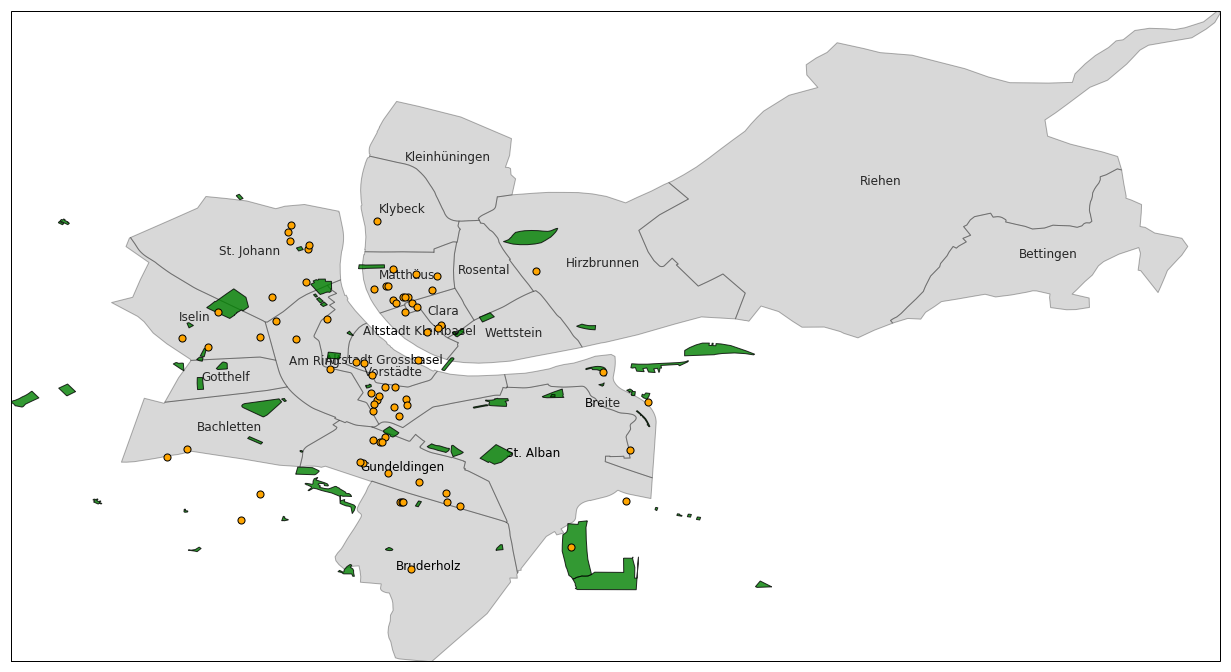
Basel's City Districts, Parks and Cafes
Data:
Basel districts shapefile from OpenStreetMap (raw data, not the .osm file).
Basel parks and cafes shapefile from BBBike.
basel_somerc = gpd.read_file(os.path.join(data_dir, 'WE_StatWohneinteilungen', 'Wohnviertel.shp'))
print(basel_somerc.crs)
basel_somerc.head()
Convert 21781 (CH1903) to 4326 (WGS84)
You can use pyproj.Proj and reproject manually...
# https://gis.stackexchange.com/a/277488/119309
input_projection = pyproj.Proj(init='EPSG:21781')
output_projection = pyproj.Proj(init='EPSG:4326')
pyproj.transform(input_projection, output_projection, x=basel_somerc.crs['x_0'], y=basel_somerc.crs['y_0'])
polygons_somerc = [basel_somerc.loc[i, 'geometry']
                   for i in range(basel_somerc.shape[0])]
polygons_wgs84 = []
for poly in polygons_somerc:
    x, y = poly.exterior.coords.xy
    x_new, y_new = pyproj.transform(input_projection, output_projection, x, y)
    poly_new = shp.geometry.Polygon(list(zip(x_new, y_new)))
    polygons_wgs84.append(poly_new)
polygons_somerc[0]
polygons_wgs84[0]
...or use GeoPandas and its to_crs method.
basel_somerc.plot()

basel_wgs84 = basel_somerc.to_crs(epsg=4326)
basel_wgs84.plot()

Add a centroid for each district
basel_wgs84['CentroidLongitude'] = basel_wgs84['geometry'].apply(lambda poly: poly.centroid.bounds[0])
basel_wgs84['CentroidLatitude'] = basel_wgs84['geometry'].apply(lambda poly: poly.centroid.bounds[1])
basel_wgs84.head()
Basel's parks
Apparently there are some issues with the shapefile I extracted from BBBike. Many shapely records are invalid.
Because of these invalid records, gv.Shape.from_shapefile does not work.
Luckily enough, you can use cartopy.shapereader.Reader and filter out these records with a simple condition.
shp_filepath = os.path.join(data_dir, 'basel_shapefiles', 'natural.shp')
reader = shpreader.Reader(shp_filepath)
parks_generator = (r for r in reader.records() if r.attributes['type'] == 'park')
parks = [p for p in parks_generator if p.geometry.area > 0]
park_geometries = [p.geometry for p in parks]
print(parks[0].attributes)
park_geometries[0]
# some parks have no name. Maybe they are just small (private?) green areas...
', '.join([p.attributes['name'] for p in parks])
%%opts Shape (fill_color='green')
gv.Shape(park_geometries[0]) * gv.Text(7.5704, 47.5653, parks[0].attributes['name'])
Basel's Cafes
shp_filepath = os.path.join(data_dir, 'basel_shapefiles', 'points.shp')
reader = shpreader.Reader(shp_filepath)
cafes = [r for r in reader.records() if r.attributes['type'] == 'cafe']
f'There are {len(cafes)} cafes in Basel'
cafes[0].geometry.bounds
cafes_data = list(map(lambda x: (x.geometry.bounds[0], x.geometry.bounds[1], x.attributes['name']), cafes))
cafes_df = pd.DataFrame(cafes_data, columns=['Longitude', 'Latitude', 'Name'])
cafes_df.head()
cafes_dataset = gv.Dataset(cafes_df, kdims=['Name'])
%%opts WMTS [width=800 height=600]
%%opts Shape (fill_color='green' fill_alpha=0.5)
%%opts Points (color='orange' line_color='black' size=7) [tools=['hover']]
hv.Overlay([
    gv.WMTS(tiles['ESRI'], crs=ccrs.PlateCarree()),
    hv.NdOverlay({i: gv.Shape(pg, crs=ccrs.PlateCarree()) for i, pg in enumerate(park_geometries)}),
    cafes_dataset.to(gv.Points, kdims=['Longitude', 'Latitude'], vdims=['Name'], crs=ccrs.PlateCarree()),
])
%%output size=600
hv.Overlay([
    hv.NdOverlay({i: shape_district(poly) for i, poly in enumerate(basel_wgs84.geometry)}),
    hv.NdOverlay({i: shape_park(poly) for i, poly in enumerate(park_geometries)}),
    hv.NdOverlay({i: text_centroid(lon, lat, name) for i, (lon, lat, name) in enumerate(list_centroid)}),
    cafe_points.opts(style={'color': 'orange', 'edgecolor': 'black', 's': 50}),
])
Districts with the highest number of Cafes?
names = []
points = []
for i, cafe in cafes_df.iterrows():
    names.append(cafe.Name)
    points.append(shp.geometry.Point((cafe.Longitude, cafe.Latitude)))

cafes_gdf = gpd.GeoDataFrame({'Cafe': names, 'geometry': points}, crs={'init': 'epsg:4326', 'no_defs': True})
cafes_gdf.head()
districts_and_cafes = gpd.sjoin(basel_wgs84[['TYPE', 'geometry']], cafes_gdf, how="left", op='contains')
# districts_and_cafes.head()
cafes_count = districts_and_cafes.groupby('TYPE')[['Cafe']].count().rename(columns={'Cafe': 'CafeCount'})
cafes_in_basel = cafes_count.sort_values(by='CafeCount', ascending=False).reset_index()
# cafes_in_basel.head()
gdf = pd.merge(basel_wgs84[['TYPE', 'geometry']], cafes_in_basel)
gdf.sort_values(by='CafeCount', ascending=False).head()
%%output size=400
%%opts Polygons (cmap='YlOrRd') [color_index='CafeCount' colorbar=True]
gv.Polygons(gdf, vdims=['TYPE', 'CafeCount'], label='Cafes in Basel districts')
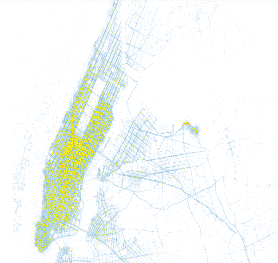
Big Data?
Use GeoViews (HoloViews) + Datashader + Matplotlib/Bokeh.
The combination HoloViews + Datashader lets you switch between Datashader and non-Datashader plots generated by Matplotlib or Bokeh.
NYC yellow taxi visualization @ hdf5-pydata-munich
Datashader
Datashader is a data rasterization pipeline similar to a 3D graphics shading pipeline.
- Projection: Data $\rightarrow$ Scene
- Aggregation: Scene $\rightarrow$ Aggregates (an aggregate bin ends up in one pixel)
- Transformation + Colormapping: Aggregates $\rightarrow$ Image
- Embedding: Image $\rightarrow$ Plot
This approach allows you to plot a lot of data, and to avoid plotting pitfalls such as:
- overplotting
- oversaturation
- undersampling
- undersaturation
- underutilized range
- nonuniform colormapping
A few resources on Datashader
PyViz: how to solve visualization problems with Python tools.
James Bednar's notebooks:
Guillem Duran Ballester's talk @ EuroPython 2017 with AirBnB data.
Johnny Chan's Bokeh app on UK road accidents.